Consider the mechanical system shown in the figure. Plot the response curve x(t) versus t with MATLAB when the mass m is pulled slightly downward, generating the initial conditions x(0)=0.05m and xdot(0)=1 m/s, and released at t=0. The displacement x is measured from the equilibrium position before m is pulled downward. Assume that m=1 kg, b1=4 Ns/m, k1=6N/m, and k2=10N/m. (a) Plot the exact solution of response for 5 s using the "residue" command. (b) Plot the response for 5 s using the "impulse" command. (c) Plot the response for 5 s using the "step" command.

Consider the mechanical system shown in the figure. Plot the response curve x(t) versus t with MATLAB when the mass m is pulled slightly downward, generating the initial conditions x(0)=0.05m and xdot(0)=1 m/s, and released at t=0. The displacement x is measured from the equilibrium position before m is pulled downward. Assume that m=1 kg, b1=4 Ns/m, k1=6N/m, and k2=10N/m. (a) Plot the exact solution of response for 5 s using the "residue" command. (b) Plot the response for 5 s using the "impulse" command. (c) Plot the response for 5 s using the "step" command.

Highalphabet Home Page dynamics dynamics System Dynamics Page 1

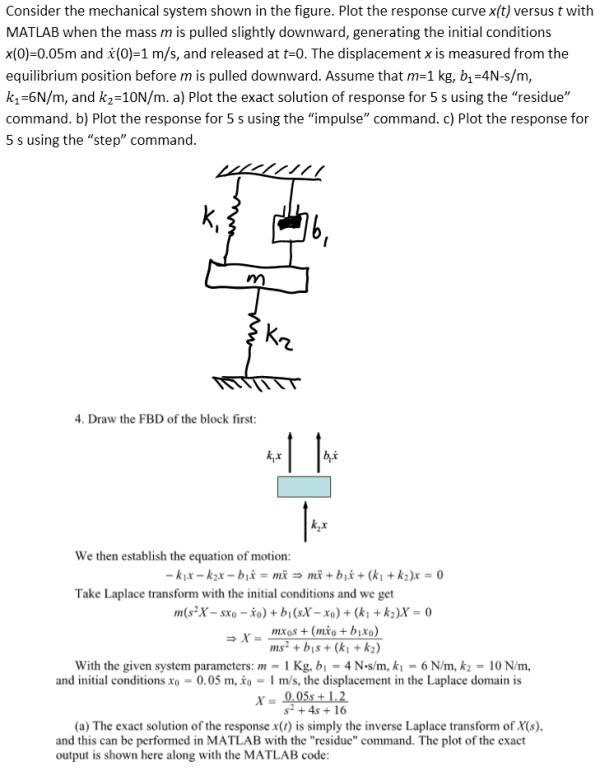
Consider the mechanical system shown in the figure. Plot the response curve x(t) versus t with MATLAB when the mass m is pulled slightly downward, generating the initial conditions x(0)=0.05m and xdot(0)=1 m/s, and released at t=0. The displacement x is measured from the equilibrium position before m is pulled downward. Assume that m=1 kg, b1=4 Ns/m, k1=6N/m, and k2=10N/m. (a) Plot the exact solution of response for 5 s using the "residue" command. (b) Plot the response for 5 s using the "impulse" command. (c) Plot the response for 5 s using the "step" command.

System Dynamics Page 2 dynamics dynamics dynamics dynamics dynamics dynamics dynamics System dynamics Page 3